 Online: 10722
Excel > Charts
2D & 3D Bubble chart in Excel
How to create 2D & 3D Bubble chart in Excel?
In last post, we learnt how to create Scatter chart in Excel. In this post, we shall learn how to create 2D and 3D Bubble chart in Excel.
2D Bubble chart
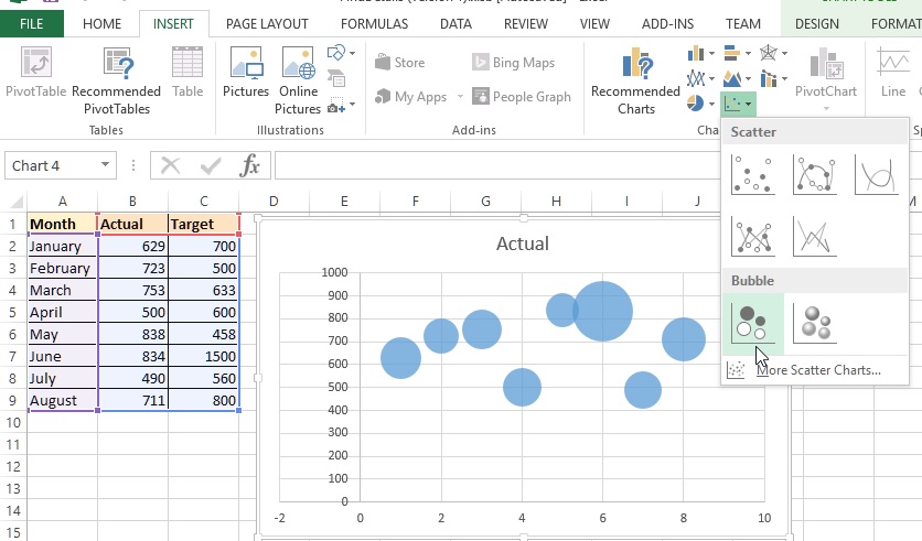
To create a Bubble chart in Excel, go to INSERT menu and click on 'Insert Scatter ...' command button on the ribbon. From the dropdown, select Bubble chart as shown below.

A Bubble chart appears for the selected data. Note that ever if you select two columns of data, the the Bubble chart displays only one column of data.
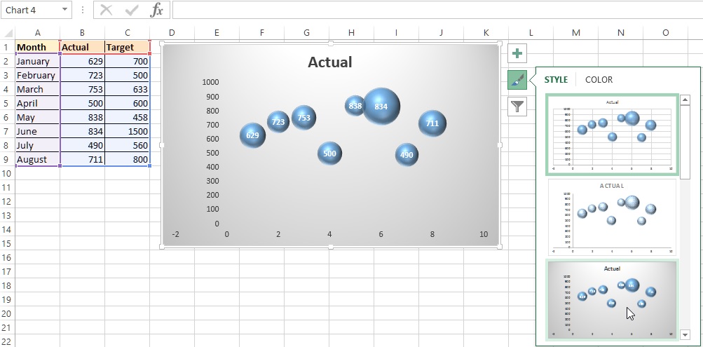
As in other charts, we can also apply style, filtering to the Bubble chart.

3D Bubble chart
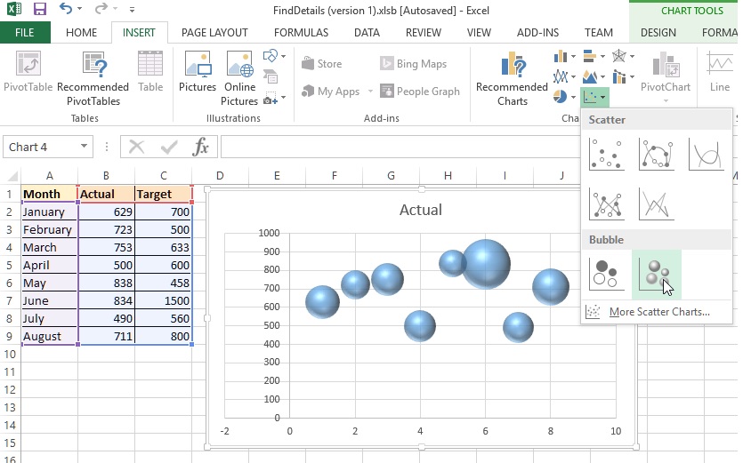
To create 3D chart, simply select the 3D version of the Bubble chart as shown below.

Thanks for reading!
Views: 15378 | Post Order: 52


