 Online: 1293


 Online: 1293
In the previous post, we learnt about Named range and Named constant. In this post we shall learn about Keyboard shortcuts in Excel.
Keyboard shortcuts are a way to perform frequently used activities quicker with the combination of keys rather than following few steps through mouse. This helps in improving the productivity of the user.
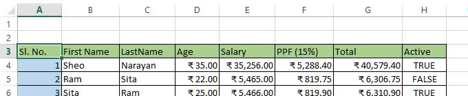
Place your mouse in any cell of data (In this case, my cursor is in A3), now press 'CTRL+A' this will select the entire range of data as shown below.

To select the entire spreadsheet, press 'CTRL+A' twice.

How to select entire row of the ranage of data in Excel?
To know basic selection of cells, rows and columns read here.
Let's assume that we have to select the header row of below data.
Select the A3 cell by clicking on it and then press 'CTRL+SHIFT+→' (CTRL+SHIFT+Right Arrow Key). The result would be

To select downwords rows, hold the SHIFT key and press ↓ key.
To select entire column of range of data (eg. A column data in this range) press 'CTRL+SHIFT+↓' (CTRL+SHIFT+Down Arrow Key).

To select right columns, hold SHIFT key and press → key.
Many a times when you may have loads of rows and columns in your spreadsheet and you want to quickly jump to the last row or last column of your data, scrolling column by column or row by row is a tough task.
To jump to the last column within range press 'CTRL+→' (CTRL+Right Arrow Key)
To jump to the last row within range press 'CTRL+↓' (CTRL+Down Arrow Key)
Similarly to go to the last cell from the range of data press 'CTRL+END', to go to the starting cell from the range of data press 'CTRL+HOME'.
Take example of below data. Go to G4 cell and press 'CTRL+=' key, hit ENTER key. This will automatically insert SUM function with range of numberic data in that row.

The same can be achieved by press Auto sum icon from Editing group on the Ribbon as shown below.

To copy the same formula to other corresponding rows of the records in the range, we can do any of following


To bring currency symbol in MS Excel, select cells either through keyboard or mouse.

Now open the Format Cells dialog box by pressing 'CTRL+1' (1 should not be pressed from Numeric keypad). Go to 'Currency' category and then in the right side from Symbol dropdown select your currency symbol.

Now press OK and here is the result.

Thanks for reading. Do share this post to your friends and colleagues.
Function Key Shortcuts
Function keys has a great benefit in Excel. Let's learn about it.
When you have not opened any dialog box and pressed F1 key, you would see a default Excel help window. This allows your search for any help or read the popular articles related wtih MS Excel.

However, if you happen to open a dialog box and need any help on that dialog box active tab then pressing F1 would open Help window box focussed to that active tab items only (Excel is intelligent, isn't it?  ).
).

For example, I had opened Format Cells dialog box and Number tab was active, when I pressed F1 here is what I see.
F2 key brings the cell into Edit mode and moves the cursor to the end of the content. If the cell contains formula, it shows the formula and selects cells on which the formula is dependent on.

F3 key brings the Paste Name dialog box provided you have already defined Named range or Named constant.

In Edit mode on the cell, it toggle through Absolute, Mixed and Related references of the cell. For example, if we have to refer D8


Pressing F6 navigates through the next split window in the spreadsheet.

Pressing F7 key opens the Spelling dialog box and gives suggestions for the content written in the selected cell.

F8 key toggles the Extended mode in the excel. Extended mode is used to select cells without dragging or pressing SHIFT key.
Press F8 and press Right Arrow key (→, any other arrow key) and you will notice that right side cells will get selected. Pressing F8 key again and pressing Right Arrow key (→, any other arrow key) again will not select cells but will select only one right side cell.

Re-evaluates all formulas of the workbook to ensure that all the cells calculated value are correct. You must have noticed that MS excel automatically evaluates the formula whenever any dependent cells value changes. However, we can change this to 'Manual' mode by going to 'Calculation Options' command from 'Calculation' group under FORMULAS tab of the Ribbon.

If the Calculation Options is selected as 'Manual', changing the dependent cells value doens't change the Formula cell (Total) value automatically.
To update the Total cells value, press F9 key.
Quickies 
Works as if ALT key is pressed on the keyboard. This shows the shortcut keys to select a particular tabs on the Ribbon.

As shown above, pressing 'M' key on the keyboard shows the 'FORMULAS' tab with the shortcuts of each command under FORMULAS tab.

Pressing F11 creates a new Chart sheet based on selected data range. In my case, I have selected LastName and Age columns.

Whe I pressed F11 key, I get a brand new sheet with chart.

It simply brings 'Save As' dialog box that allows us to duplicate the file and save with a different name.

Thanks for reading. If you liked it, do share with your friends and colleagues.