---

Search posts under Excel:

---

Pivot Table Items Grouping in Excel

How to group Pivot Table items in MS Excel?

In last post, we learnt how to create Pivot Table and Pivot Chart. In this post, we shall learn how to group Pivot Table items. It is used to combine similar types of items in a group and see the result.

Grouping Pivot Table Items

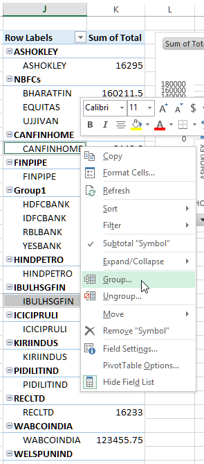
Below is the Pivot Table created using last post. In this table, you can see that there are more than one companies belongs to Banks categories.

What if we want to see Pivot Table & Pivot Chart for all bank as a whole, in this case we can using Pivot Table Items grouping.

To group Items in Pivot Table, select all banks by holding the CTRL key and clicking on Bank names. Now right click and select 'Group...'.

This will bring the Pivot Table grouped by Banks however notice that the name of the group appears as 'Group1' by default.

To change the Group name, simply click on the Group name and go to Formula bar and edit the name as I have done it below.

Creating multiple group items in Pivot Table

To create more such groups, follow the same steps. Select multiple items of similar categories and right click to select 'Group...'.

You can click on - icon to collapse group icons and vice-versa.

If you have a Pivot Chart created for Pivot Table, it also changes in real time.

Thanks for reading, hope this was informative. Please share if you liked it.