---

Search posts under Excel:

---

Calculate monthly installment of a loan in Excel

How to calculate payment for a loan based on constant payment and interest rate in Excel?

In the last post, we learnt about getting maximum and minimum value from set of values in Excel. In this post, we shall learn how to calculate payment for a loan based on monthly payment and to a specific interest rate. This can be done using PMT function of Excel.

To understand how it works, we shall calculate the monthly payment of a term loan of 14,50,000 for a period of 20 years on 9.75% interest rate.

PMT function 

Get monthly installments for loan

The PMT function helps in getting payment amount (installment) of a loan. It accepts at least 3 parameters and they are

1. rate - interest rate, as the yearly interest rate is 9.75 so monthly will be (0.75/12)% ie. 0.008125.
   
   
2. nper - total number of periods, as the payment term is monthly so total pay period will be 20*12 ie. 240.
   
   
3. pv - present value, total amount borrowed ie. 14,50,000
   
   
4. [fv] (Optional) - the future value of the loan, we want to completely pay off so it will be 0
   
   

The same calculation if we do for Nper 180 (ie. 15 years) we get different result (notice 3rd row). Just for the sake of knowing how much you end up paying more, we have kept the F and G column.

RATE function

Get interest rate of the loan

Similar to above, if we want to know what would be the interest rate, if we want to borrow certain amount, for certain period of time and we want to pay a certain amount every month then we can use RATE function.

In B4 cell, we have '=RATE(C2,A2, D2, E2)' formula where

• C2 is Nper (number of months we want to pay)
• A2 is monthly payment we want to make
• D2 is the amount of money we want to borrow
• E2 is the value left after paying

The result would look like this. In general result come in full number, simply use cell formatting to display decimal numbers.

NPER function

Get period (in months) of a loan

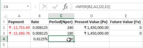
Let's say we want to know the period (in months) we will have to pay if we borrow certain amount at certain interest rate and we want to pay certain amount every month, then we can use NPER function.

In C4 cell, we have '=NPER(B2,A2,D2,E2)' formula where

• B2 is rate of interest
• A2 is monthly installment we want to pay
• D2 is amount we want to borrow
• E2 is the amount left after paying installments

PV function

Get how much we can borrow

Let's assume that you want to know that if you pay certain amount every month, till certain period of months with certain interest rate then how much amount you can borrow? We will need to use PV function.

In D4 cell we have '=PV(B2,C2,A2,E2)' formula where

• B2 is the rate of interest
• C2 is the number of months we want to pay
• A2 is the amount we want to pay every month
• E2 is the left over amount after paying

FV function

Get if you can pay off loan after paying only certain amount every month

Let's assume a scenario where you want to know that what if you pay only certain amount every month, with a certain interest rate for a certain amount of loan, whether you will be able to pay off the entire loan? To know this we can use FV function

In E4 cell, we have '=FV(B2,C2, A2,D2)' formula where

• B2 is the loan rate of interest 
• C2 is the period in months we want to repay
• A2 is the amount we are willing to pay every month
• D2 is the loan amount we want to borrow

Notice that slight change (only 753.49 less amount) in the Payment amount (installment) results in huge left over amount (5,53,971.31).

Here you must be knowing the magic of cummulative interest. The same applies when you save money every month !